Here is one for the functional safety nerds. I find that every time I study the diagrams for 1oo2 Architecture and the matching equations I realize some new insights. I have tried to capture some of my understanding and insights in the blog below. I am sure there is more I have missed and when I next come back and look at it there will be more to be discovered.
IEC 61508-6:2010 Annex B analyses how to calculate the probability of failure calculations for several architectures including the 1oo2 architecture. In this case 1oo2 stands for “one out of two” which means there are two safety channels with each channel arranged so that if at least one of them trips the system will go to the safe state. This typically gives a higher level of safety than having a single channel. I say typically because a single channel architecture with very reliable components and/or a higher level of diagnostic coverage could achieve a lower PFH.
The block diagram for a 1oo2 channel from IEC 61508-6:2010 figure B.6 is redrawn is below.
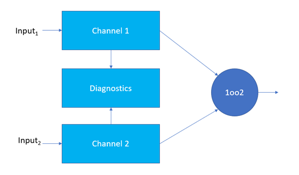
Figure 1 – a 1oo2 architecture from IEC 61508
This drawing matches the text from B.3.2.2.2 which states “This architecture consists of two channels connected in parallel, such that either channel can process the safety function. Thus, there would have to be a dangerous failure in both channels before a safety function failed on demand.” (Reference: IEC 61508-6:2010)
The darker blue square containing the 1oo2 text is a voter and I think the architecture would be better shown as something like the below for clarity because otherwise the vote itself is a single point of failure defeating the redundancy.
Here the voting logic is shown as two switches. If either of the switches opens the power is removed from the actuator or contactor which brings the machine to the safe state (removal of power is often referred to as a basic safety measure).
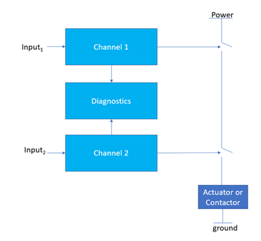
Figure 2 – 1oo2 redrawn for clarity on the voter
Before anybody asks why wouldn’t there be a third output for the diagnostics to control an additional switch the text makes it clear that “It is assumed that any diagnostic testing would only report the faults found and would not change any output states or change the output voting” so the diagram and the text are consistent. It could also be changed to have an additional block of diagnostics per channel rather than a shared diagnostic block but tis but this is clearly not done. As we will see later the equations assume identical redundancy (only 1 common value of DC and λDU for both channels). The diagnostics could be diagnostics by comparison in which case while the system will go to the safe state you have no way to tell which of the channels had a failure.
I note the 1oo2D architecture has a diagnostic block per channel and the diagnostics do feed into the voting but be careful because the 1oo2D architecture as drawn in IEC 61508-6:2010 is actually optimized for high availability with somewhat higher safety as evidenced by its description which states “During normal operation, both channels need to demand the safety function before it can take place”. I have seen other documents and standards which have a different meaning for 1oo2D.
A matching reliability block diagram for the 1oo2 architecture is given in figure B.7 of IEC 61508-6. I have redrawn it below.
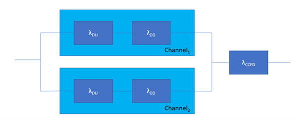
Figure 3 – Reliability block diagram for 1oo2 architecture
A reliability block diagram is a tool to evaluate PFH (probability of dangerous failure per hour average) for a safety function. In this diagram only the dangerous failure rates for each channel and a common cause contribution is shown.
Each channel can fail dangerously or safely but safe or indeed no effect failures are not shown on the reliability block diagram. Instead only dangerous undetected failures and dangerous detected failures are shown and represented by λDU and λDD. In addition, a common cause failure contribution is shown in series with the parallel channels with its dangerous failure rate represented by λCCFD. Common cause failures are failures which cause both channels to fail at the same time (as distinct for random failures in either of the channels separately).
If you are paying attention you might ask why are the dangerous detected failures included. These failures are detected but the information is not used in a 1oo2 architecture as defined in Annex B as it clearly states “It is assumed that any diagnostic testing would only report the faults found and would not change any output states or change the output voting.”. This I feel is unusual and would make the resulting equations conservative if your system actually has a means to go to a safe state for dangerous detected failures.
It is not clear from the description of the 1oo2 architecture however the equations which we will study later make it clear that the detected failures are somehow flagged to a repair team who will fix the detected errors in time MTTR. Until these repairs are made the system operates with a lower integrity using the good channel. This gives a higher level of availability than if the diagnostics had their own output to take the system to a safe state.
I note the equation doesn’t model the failure rate of the diagnostics but this isn’t included even in the calculation for a 1oo1 system and for me at least it is unclear as to whether a failure of the diagnostics corresponds to a dangerous failure of the safety function according to IEC 61508 and the requirement to model them according to revision 2 of IEC 61508 is restricted to a statement in Annex D of part 2 saying the safety manual must contain a failure rate for the diagnostics. Anyway I digress to lets get back to the equation.
We now jump from the low demand section of IEC 61508 part 6 to the high demand section in B.3.3.2.2 where we find the equation below.
![]()
Figure 4 – average probability of dangerous failure per hour for a 1oo2 architecture
The equation includes:
- βD– the proportion of detected failures that causes both channels to fail at the same time. Typical values are 0.01, 0.02 to 0.1.
- β – the proportion of all failure that causes both channels to fail at the same time. Typical values are similar to those for β.
- λDD – the rate of dangerous detected failures for each of the channels. Values are often in the range of 1e-6 to 1e-9/h.
- λDU– the rate of dangerous undetected failures for each of the channels. Values are often in the range of 1e-6 to 1e-9/h.
- TCE – see below
The definition of tCE is given in the 1oo1 section as shown below so let’s start with it.
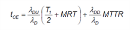
Figure 5 – channel equivalent down time
Here there are some new terms:
- T1– the proof test interval or if no proof testing the expected operating lifetime of the safety system. T1 is given in hours where a year is 8760 hours.
- MRT – Mean repair time in hours
- MTTR – Mean time to restoration in hours
Both MRT and MTTR are repair times but one applies to the failures detected by proof tests and the others to failures by automatic tests (i.e. the normal diagnostics).
So, let’s start with tCE which has two parts.
The first part of the tCE equation represents the fraction of dangerous failures which are undetected by any automatic diagnostics. If a non-automatic test (a proof test) is performed it is assumed that this will detect the failures not detected by the automatic tests and that on average these failures will have existed for T1/2 + the time to implement the repair. In practice, T1 is often equal to the expected lifetime of the system since no proof test is ever completed. On average the failure will have existed for half the lifetime in that case. When a failure is detected by proof testing it is repair in MRT.
The second half of the tCE equation represents the dangerous detected failures and once detected they are repaired in MTTR. In practice you can probably set MRT=MTTR=0 on the assumption that repair times are fast compared to the lifetime of the system (offshore windfarms or space applications might not benefit from this assumption). While down and awaiting repair, the system is relying on the other channel being functional.
So now let’s go back to the main equation.
![]()
Figure 6 – repeat of the equation from the standard
Let’s take the last bit of the equation first. βλDU = λCCFD from the reliability block diagram. Typical values for β are 1%, 2%, 5% or 10%. If β=10% then PFHG is typically 10% of the dangerous undetected failure rate for a single channel i.e. the reliability (in a safety sense) of the channel is improved by a factor of 10. Without this portion of the equation you would naively assume that the FIT rate was 100x, 1000x improved or even more.
The first part of the equation represents an accumulation of undetected failures which on average will exist for T1/2 where T1 is the proof test interval or the lifetime of the safety system whichever is less. To see this let’s set MTTR=MTR=β=βD=0. The first part of the equation then becomes PFHG = 2λDU2T1/2 where the λDU2 represents the probability of two completely independent items failing and the first 2 is included because there are two ways this can happen with channel 1 failure first and then channel 2 or vice-versa. The T1/2 at the end comes from the fact that if a failure exists it will on average exist for T1/2 (remember PFH standards for average probability of dangerous failure per hour).
If you want to get a feeling for the results the equations gives for various values of the input variables the subsequent tables B.10 to B.13 give the calculated PFHG for various architectures as λD, DC, β, MTTR and T1 are varied with the assumption that βD=β/2.
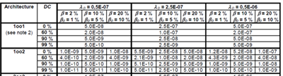
Figure 7 – some pre-calculated values from IEC 61508-6:2010
Breaking the equation into multiple parts it is interesting to look at which part of the equation dominates.
With a proof test interval of 20 years, MTTR=MTR=0, β=0.02, λD=50 the first part of the equation is a maximum of < 20% of the total for DC=60% and becomes rapidly less significant as the DC increases.
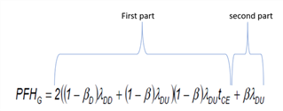
Figure 8 – equation in parts
Once the proof test interval drops to 10 years and less the first part of the equation becomes insignificant.
As Beta reduces to 2% or less the impact of the first half of the equation becomes more significant but is still less than 30% of the total for the minimum viable values of β which to me is counter intuitive. I must try and find time to play with this equation again.
As regards where this equation comes from, I don’t know. But I have seen some papers on similar equations and an extract is shown below. I have tried to derive it for myself using a Markov model and a symbolic math program but lost patience before I could figure out how to do integration by parts in the math software. Below is the middle of one derivation I have seen showing steps 95 to 98 in the derivation so you would need good mathematical knowledge and a lot of time to verify this equation from first principles.
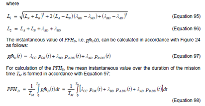
Figure 9 – example of the calculations behind the equations
While on the subject of equations my favourite equation is Euler’s identity. It has all the key mathematical symbols in one equation. I’m not aware however of any practical application of this equation in functional safety. You can however buy a mug with this equation on Amazon to impress your work colleagues!
Figure 10 – Euler’s identity

The post Musing on a 1002 Architecture appeared first on ELE Times.
No comments:
Post a Comment